parametric Archives • Statisticelle

Parametric statistics assume that the unknown CDF $F$ belongs to a family of CDFs characterized by a parameter (vector) $\theta$ . As the form of $F$ is assumed, the target of estimation is its parameters $\theta$ . Thus, all uncertainty about $F$ is comprised of uncertainty about its parameters. Parameters are estimated by $\hat{\theta}$ , and estimates are be substituted into the assumed distribution to conduct inference for the quantities of interest. If the assumed distribution $F$ is incorrect, inference may also be inaccurate, or trends in the data may be missed.

To demonstrate the parametric approach, consider $n = 100$ independent and identically distributed random variables $X_1, …, X_n$ generated from an exponential distribution with rate $\lambda = 2$ . Investigators wish to estimate the 75 $^{th}$ percentile and erroneously assume that their data is normally distributed. Thus, $F$ is assumed to be the Normal CDF but $\mu$ and $\sigma^2$ are unknown. The parameters $\mu$ and $\sigma$ are estimated in their typical way by $\bar{x}$ and $\sigma^2$ , respectively. Since the normal distribution belongs to the location-scale family, an estimate of the $p^{th}$ percentile is provided by,

$x_p = \bar{x} + s\Phi^{-1}(p)$

where $\Phi^{-1}$ is the standard normal quantile function, also known as the probit.

set.seed(12345)
library(tidyverse, quietly = T)

# Generate data from Exp(2)
x <- rexp(n = 100, rate = 2)

# True value of 75th percentile with rate = 2
true <- qexp(p = 0.75, rate = 2) 
true

## [1] 0.6931472

# Estimate mu and sigma
xbar <- mean(x)
s    <- sd(x)

# Estimate 75th percentile assuming mu = xbar and sigma = s
param_est <- xbar + s * qnorm(p = 0.75)
param_est

## [1] 0.8792925

The true value of the 75 $^{th}$ percentile of $\text{Exp}(2)$ is 0.69 while the parametric estimate is 0.88.

Nonparametric statistics make fewer distributions about the unknown distribution $F$ , requiring only mild assumptions such as continuity or the existence of specific moments. Instead of estimating parameters of $F$ , $F$ itself is the target of estimation. $F$ is commonly estimated by the empirical cumulative distribution function (ECDF) $\hat{F}$ ,

$\hat{F}(x) = \frac{1}{n} \sum_{i=1}^{n} \mathbb{I}(X_i \leq x).$

Any statistic that can be expressed as a function of the CDF, known as a statistical functional and denoted $\theta = T(F)$ , can be estimated by substituting $\hat{F}$ for $F$ . That is, plug-in estimators can be obtained as $\hat{\theta} = T(\hat{F})$ .

Continue reading Parametric vs. Nonparametric Approach to Estimations

Motivation

For observed pairs $(x_i, y_i)$ , $i = 1, …, n$ , the relationship between $x$ and $y$ can be defined generally as

$y_i = m(x_i) + \varepsilon_i$

where $f(x_i) = E[y_i | x = x_i]$ and $\varepsilon_i \stackrel{iid}{\sim} (0, \sigma^2)$ . If we are unsure about the form of $m(\cdot)$ , our objective may be to estimate $m(\cdot)$ without making too many assumptions about its shape. In other words, we aim to “let the data speak for itself”.

Simulated scatterplot of $y = f(x) + \epsilon$ . Here, $x \sim Uniform(0, 10)$ and $\epsilon \sim N(0, 1)$ . The true function $f(x) = sin(x)$ is displayed in green.

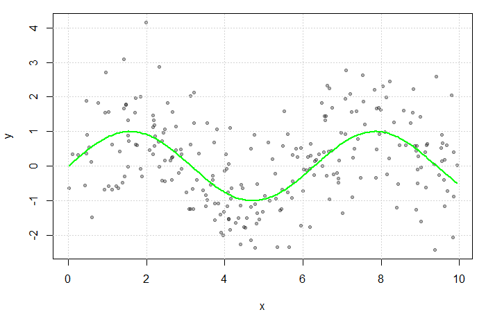
Non-parametric approaches require only that $m(\cdot)$ be smooth and continuous. These assumptions are far less restrictive than alternative parametric approaches, thereby increasing the number of potential fits and providing additional flexibility. This makes non-parametric models particularly appealing when prior knowledge about $m(\cdot)$ ‘s functional form is limited.

Estimating the Regression Function

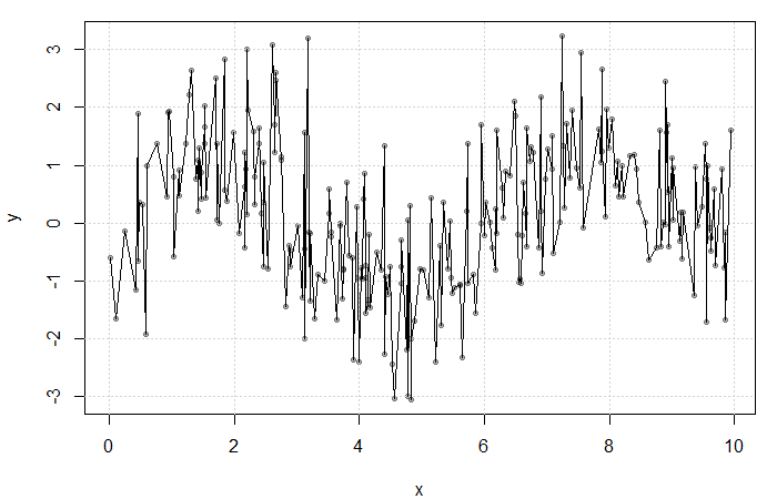
If multiple values of $y$ were observed at each $x$ , $f(x)$ could be estimated by averaging the value of the response at each $x$ . However, since $x$ is often continuous, it can take on a wide range of values making this quite rare. Instead, a neighbourhood of $x$ is considered.

Result of averaging $y_i$ at each $x_i$ . The fit is extremely rough due to gaps in $x$ and low $y$ frequency at each $x$ .

Define the neighbourhood around $x$ as $x \pm \lambda$ for some bandwidth $\lambda > 0$ . Then, a simple non-parametric estimate of $m(x)$ can be constructed as average of the $y_i$ ‘s corresponding to the $x_i$ within this neighbourhood. That is,

(1) $\begin{equation*} \hat{f}_{\lambda}(x) = \frac{\sum_{n} \mathbb{I}(|x - x_i| \leq \lambda)~ y_i}{\sum_{n} \mathbb{I}(|x - x_i| \leq \lambda)} = \frac{\sum_n K\left( \frac{x - x_i}{\lambda} \right) y_i}{\sum_n K\left( \frac{x - x_i}{\lambda} \right) } \end{equation*}$

where

$K(u) = \begin{cases} \frac{1}{2} & |u| \leq 1 \\ 0 & \text{o.w.} \end{cases}$

is the uniform kernel. This estimator, referred to as the Nadaraya-Watson estimator, can be generalized to any kernel function $K(u)$ (see my previous blog bost). It is, however, convention to use kernel functions of degree $\nu = 2$ (e.g. the Gaussian and Epanechnikov kernels).

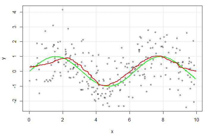
The red line is the result of estimating $f(x)$ with a Gaussian kernel and arbitrarily selected bandwidth of $\lambda = 1.25$ . The green line represents the true function $sin(x)$ .

Tag: parametric

Parametric vs. Nonparametric Approach to Estimations

Kernel Regression

Motivation

Estimating the Regression Function