Kernel Regression

Motivation

For observed pairs $(x_i, y_i)$ , $i = 1, …, n$ , the relationship between $x$ and $y$ can be defined generally as

$y_i = m(x_i) + \varepsilon_i$

where $f(x_i) = E[y_i | x = x_i]$ and $\varepsilon_i \stackrel{iid}{\sim} (0, \sigma^2)$ . If we are unsure about the form of $m(\cdot)$ , our objective may be to estimate $m(\cdot)$ without making too many assumptions about its shape. In other words, we aim to “let the data speak for itself”.

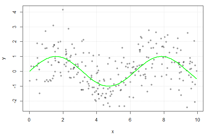
Simulated scatterplot of $y = f(x) + \epsilon$ . Here, $x \sim Uniform(0, 10)$ and $\epsilon \sim N(0, 1)$ . The true function $f(x) = sin(x)$ is displayed in green.

Non-parametric approaches require only that $m(\cdot)$ be smooth and continuous. These assumptions are far less restrictive than alternative parametric approaches, thereby increasing the number of potential fits and providing additional flexibility. This makes non-parametric models particularly appealing when prior knowledge about $m(\cdot)$ ‘s functional form is limited.

Estimating the Regression Function

If multiple values of $y$ were observed at each $x$ , $f(x)$ could be estimated by averaging the value of the response at each $x$ . However, since $x$ is often continuous, it can take on a wide range of values making this quite rare. Instead, a neighbourhood of $x$ is considered.

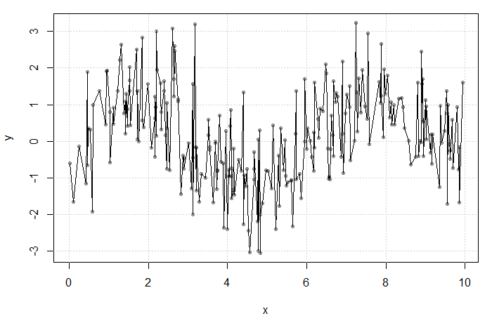
Result of averaging $y_i$ at each $x_i$ . The fit is extremely rough due to gaps in $x$ and low $y$ frequency at each $x$ .

Define the neighbourhood around $x$ as $x \pm \lambda$ for some bandwidth $\lambda > 0$ . Then, a simple non-parametric estimate of $m(x)$ can be constructed as average of the $y_i$ ‘s corresponding to the $x_i$ within this neighbourhood. That is,

(1) $\begin{equation*} \hat{f}_{\lambda}(x) = \frac{\sum_{n} \mathbb{I}(|x - x_i| \leq \lambda)~ y_i}{\sum_{n} \mathbb{I}(|x - x_i| \leq \lambda)} = \frac{\sum_n K\left( \frac{x - x_i}{\lambda} \right) y_i}{\sum_n K\left( \frac{x - x_i}{\lambda} \right) } \end{equation*}$

where

$K(u) = \begin{cases} \frac{1}{2} & |u| \leq 1 \\ 0 & \text{o.w.} \end{cases}$

is the uniform kernel. This estimator, referred to as the Nadaraya-Watson estimator, can be generalized to any kernel function $K(u)$ (see my previous blog bost). It is, however, convention to use kernel functions of degree $\nu = 2$ (e.g. the Gaussian and Epanechnikov kernels).

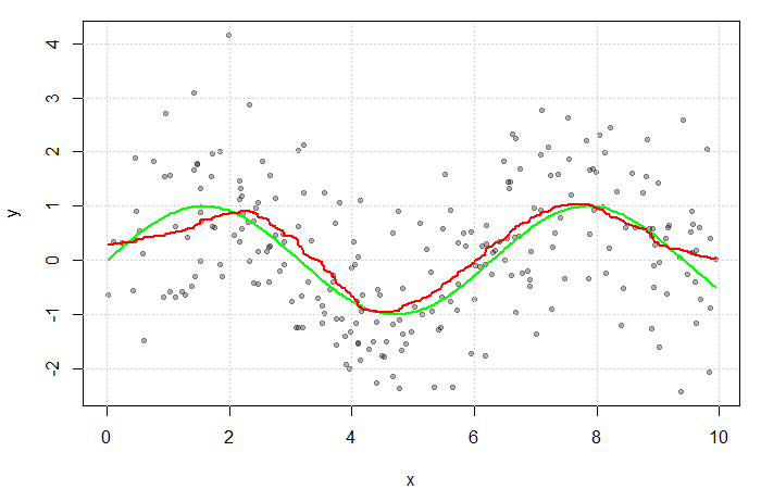
The red line is the result of estimating $f(x)$ with a Gaussian kernel and arbitrarily selected bandwidth of $\lambda = 1.25$ . The green line represents the true function $sin(x)$ .

Kernel and Bandwidth Selection

The implementation of a kernel estimator requires two choices:

the kernel, $K(u)$ , and
the smoothing parameter, or bandwidth, $\lambda$ .

Kernels are often selected based on their smoothness and compactness. We prefer a compact kernel to ensure that only data local to the point of interest is considered. The optimal choice, under some standard assumptions, is the Epanechnikov kernel. This kernel has the advantages of some smoothness, compactness, and rapid computation.

The choice of bandwidth $\lambda$ is critical to the estimator’s performance and far more important than the choice of kernel. If the smoothing parameter is too small, the estimator will be too rough; but if it is too large, we risk smoothing out important function features. In other words, choosing $\lambda$ involves a significant bias-variance trade-off.

$\lambda \uparrow ~~~\Rightarrow$ smooth curve, low variance, high bias
$\lambda \downarrow ~~~\Rightarrow$ rough curve, high variance, low bias

The simplest way of selecting $\lambda$ is to plot $\hat{m}_\lambda(x)$ for a range of different $\lambda$ and pick the one that looks best. The eye can always visualize additional smoothing, but it is not easy to imagine what a less smooth fit might look like. For this reason, it is recommended that you choose the least smooth fit that does not show any implausible fluctuations.

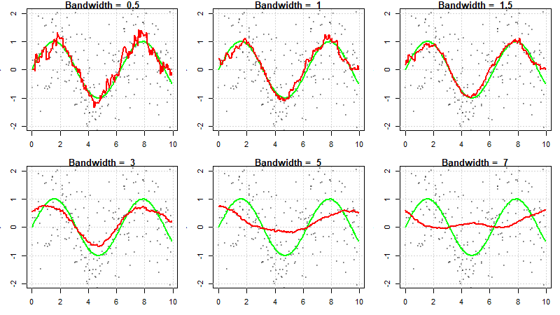
Kernel regression fits for various values of $\lambda$ .

Cross-Validation Methods

Selecting the amount of smoothing using subjective methods requires time and effort. Automatic selection of $\lambda$ can be done via cross-validation. The cross-validation criterion is

$CV(\lambda) = \frac{1}{n} \sum_{n} \left( y_j - \hat{m}_{\lambda}^{(-j)} x_j \right)^2$

where $(-j)$ indicates that point $j$ is left out of the fit. The basic idea is to leave out observation $j$ and estimate $m(\cdot)$ based on the other $n-1$ observations. $\lambda$ is chosen to minimize this criterion.

True cross-validation is computationally expensive, so an approximation known as generalized cross-validation (GCV) is often used. GCV approximates CV and involves only one non-parametric fit for each $\lambda$ value (compared to CV which requires $n$ fits at each $\lambda$ ).

In order to approximate CV, it is important to note that kernel smooths are linear. That is,

$\hat{Y} = \hat{m}_{\lambda}(x) = S_{\lambda} y$

where $S_{\lambda}$ is an $n \times n$ smoothing matrix. $S_{\lambda}$ is analogous to the hat matrix $H$ in parametric linear models.

$H = X(X^{T}X)^{-1}X^{T}$

It can be shown that

$CV(\lambda) = \frac{1}{n} \sum_{n} \left[ \frac{y_i - \hat{m}_{\lambda}(x_i)}{1 - s_{ii}(\lambda)} \right]^2$

where $s_{ii}(\lambda)$ is the $i^{th}$ diagonal element of $S_{\lambda}$ (hence $s_{ii}$ is analogous to $h_{ii}$ , the leverage of the $i^{th}$ observation). Using the smoothing matrix,

$GCV(\lambda) = \frac{1}{n} \sum_{i=1}^{n} \left[ \frac{y_i - \hat{m}_{\lambda}(x_i)}{1 - \frac{\text{tr}(S_{\lambda})}{n}}\right]$

where $\text{tr}(S_{\lambda})$ is the trace of $S_{\lambda}$ . In this sense, GCV is analogous to the influence matrix.

Automatic methods such as CV often work well but sometimes produce estimates that are clearly at odds with the amount of smoothing that contextual knowledge would suggest. Therefore, it is essential to exercise caution when using them, and it is recommended that they be used as a starting point.

Download this blog post as an RMarkdown (.Rmd) file!

Motivation

Estimating the Regression Function

Kernel and Bandwidth Selection

Cross-Validation Methods

Published by

Emma Davies Smith

Leave a Reply Cancel reply