Embracing the EM algorithm: One continuous response

Overview

I’m currently working on a project that revolves around the EM algorithm, and am finally realizing the power of this machinery. It really is like that movie with Jim Carrey where he can’t stop seeing the number 23 everywhere, except for me it’s the EM algorithm. Apparently this is called THE BAADER-MEINHOF PHENOMENON, oooh that’s fancy. You’ve probably seen the EM algorithm around too – though perhaps you didn’t know it. It’s commonly used for estimation with missing data. A modified EM algorithm (EMis) is used by the Amelia library in R. The EM algorithm also underpins latent variable models, which makes sense because latent variables are really missing observations when you think about it, right?! The more I learn about statistics, the more I realize most things are really missing data problems… cough potential outcomes cough

Anyways, I was previously taught the EM algorithm using the classic multinomial example. This is a great teaching tool, but I’ve never run into a situation like this in my life (yet). But, I do run into mixture distributions a surprising amount – mostly when investigating heterogeneity within patient populations. There’s a whole textbook on this, see: Medical Applications of Finite Mixture Models. The EM algorithm makes a lot more sense to me in the context of mixture models:

We sample a group of patients and observe their response.
We notice a bimodal structure in the response distribution.
We hypothesize the observed distribution actually corresponds to two subpopulations or “classes.”
We don’t know who belongs to which subpopulation.
We estimate the probability of latent class membership using the EM algorithm.

Wouldn’t ya know it, this is unsupervised clustering.

In this blog post, I motivate the EM algorithm in the context of a two-component Gaussian mixture model. A thorough walkthrough of the underlying theory is provided. In this case, estimators take a nice closed form, but this is rarely the case for complex problems encountered in practice. R code for implementating the EM algorithm using the closed form estimators is provided. I also demonstrate how this model can be easily fit using the flexmix library.

Figure: A two-component Gaussian mixture density.

Continue reading Embracing the EM algorithm: One continuous response

Kernel Regression

Motivation

For observed pairs $(x_i, y_i)$ , $i = 1, …, n$ , the relationship between $x$ and $y$ can be defined generally as

$y_i = m(x_i) + \varepsilon_i$

where $f(x_i) = E[y_i | x = x_i]$ and $\varepsilon_i \stackrel{iid}{\sim} (0, \sigma^2)$ . If we are unsure about the form of $m(\cdot)$ , our objective may be to estimate $m(\cdot)$ without making too many assumptions about its shape. In other words, we aim to “let the data speak for itself”.

Simulated scatterplot of $y = f(x) + \epsilon$ . Here, $x \sim Uniform(0, 10)$ and $\epsilon \sim N(0, 1)$ . The true function $f(x) = sin(x)$ is displayed in green.

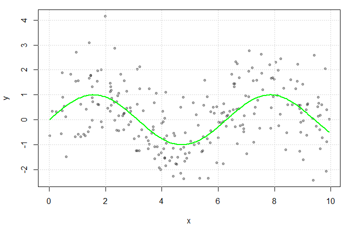
Non-parametric approaches require only that $m(\cdot)$ be smooth and continuous. These assumptions are far less restrictive than alternative parametric approaches, thereby increasing the number of potential fits and providing additional flexibility. This makes non-parametric models particularly appealing when prior knowledge about $m(\cdot)$ ‘s functional form is limited.

Estimating the Regression Function

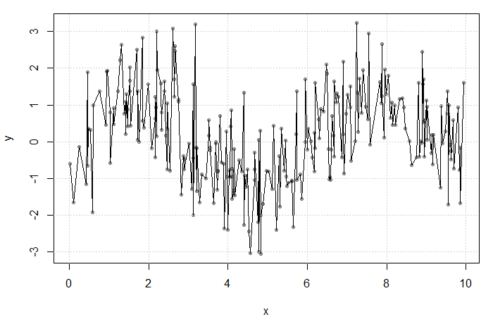
If multiple values of $y$ were observed at each $x$ , $f(x)$ could be estimated by averaging the value of the response at each $x$ . However, since $x$ is often continuous, it can take on a wide range of values making this quite rare. Instead, a neighbourhood of $x$ is considered.

Result of averaging $y_i$ at each $x_i$ . The fit is extremely rough due to gaps in $x$ and low $y$ frequency at each $x$ .

Define the neighbourhood around $x$ as $x \pm \lambda$ for some bandwidth $\lambda > 0$ . Then, a simple non-parametric estimate of $m(x)$ can be constructed as average of the $y_i$ ‘s corresponding to the $x_i$ within this neighbourhood. That is,

(1) $\begin{equation*} \hat{f}_{\lambda}(x) = \frac{\sum_{n} \mathbb{I}(|x - x_i| \leq \lambda)~ y_i}{\sum_{n} \mathbb{I}(|x - x_i| \leq \lambda)} = \frac{\sum_n K\left( \frac{x - x_i}{\lambda} \right) y_i}{\sum_n K\left( \frac{x - x_i}{\lambda} \right) } \end{equation*}$

where

$K(u) = \begin{cases} \frac{1}{2} & |u| \leq 1 \\ 0 & \text{o.w.} \end{cases}$

is the uniform kernel. This estimator, referred to as the Nadaraya-Watson estimator, can be generalized to any kernel function $K(u)$ (see my previous blog bost). It is, however, convention to use kernel functions of degree $\nu = 2$ (e.g. the Gaussian and Epanechnikov kernels).

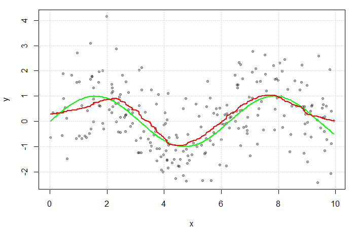
The red line is the result of estimating $f(x)$ with a Gaussian kernel and arbitrarily selected bandwidth of $\lambda = 1.25$ . The green line represents the true function $sin(x)$ .

Continue reading Kernel Regression

Kernel Density Estimation

Motivation

It is important to have an understanding of some of the more traditional approaches to function estimation and classification before delving into the trendier topics of neural networks and decision trees. Many of these methods build on an understanding of each other and thus to truly be a MACHINE LEARNING MASTER, we’ve got to pay our dues. We will therefore start with the slightly less sexy topic of kernel density estimation.

Let $X$ be a random variable with a continuous distribution function (CDF) $F(x) = Pr(X \leq x)$ and probability density function (PDF)

$f(x) = \frac{d}{dx} F(x)$

Our goal is to estimate $f(x)$ from a random sample $\lbrace X_1, …, X_n \rbrace$ . Estimation of $f(x)$ has a number of applications including construction of the popular Naive Bayes classifier,

$\hat{Pr}(C = c | X = x_0) = \frac{\hat{\pi}_c \hat{f}_{c}(x_0)}{\sum_{k=1}^{C} \hat{\pi}_{k} \hat{f}_{k}(x_0)}$

Continue reading Kernel Density Estimation