Motivation
For observed pairs  ,
,  , the relationship between
  and
and  can be defined generally as
![\[ y_i = m(x_i) + \varepsilon_i \]](https://statisticelle.com/wp-content/ql-cache/quicklatex.com-78fa8d7d51d22115d6a1fe5a2c1bdf3b_l3.png "Rendered by QuickLaTeX.com")
where ![f(x_i) = E[y_i | x = x_i]](https://statisticelle.com/wp-content/ql-cache/quicklatex.com-cce0672391a02b3395ffd209d0d01d74_l3.png "Rendered by QuickLaTeX.com") and
and  . If we are unsure about the form of
  , our objective may be to estimate without making too many assumptions about its shape. In other words, we aim to “let the data speak for itself”.
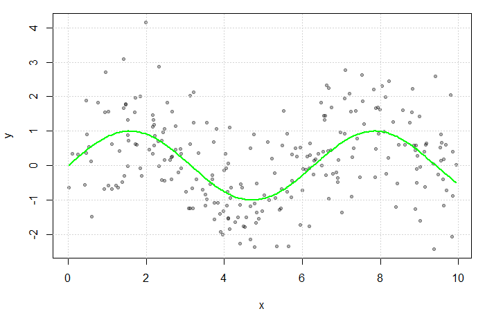
Simulated scatterplot of  . Here,
  and
and  . The true function
  is displayed in green.
Non-parametric approaches require only that be smooth and continuous. These assumptions are far less restrictive than alternative parametric approaches, thereby increasing the number of potential fits and providing additional flexibility. This makes non-parametric models particularly appealing when prior knowledge about ‘s functional form is limited.
Estimating the Regression Function
If multiple values of were observed at each ,  could be estimated by averaging the value of the response at each . However, since is often continuous, it can take on a wide range of values making this quite rare. Instead, a neighbourhood of is considered.
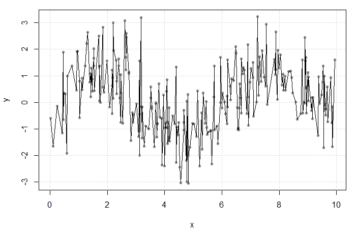
Result of averaging  at each
  . The fit is extremely rough due to gaps in and low frequency at each .
Define the neighbourhood around as  for some bandwidth
  . Then, a simple non-parametric estimate of
  can be constructed as average of the ‘s corresponding to the within this neighbourhood. That is,
(1) 
where
![\[ K(u) = \begin{cases} \frac{1}{2} & |u| \leq 1 \\ 0 & \text{o.w.} \end{cases} \]](https://statisticelle.com/wp-content/ql-cache/quicklatex.com-27c264e157b25fba34a6f4f7702c9ce2_l3.png "Rendered by QuickLaTeX.com")
is the uniform kernel. This estimator, referred to as the Nadaraya-Watson estimator, can be generalized to any kernel function  (see my previous blog bost). It is, however, convention to use kernel functions of degree
  (e.g. the Gaussian and Epanechnikov kernels).
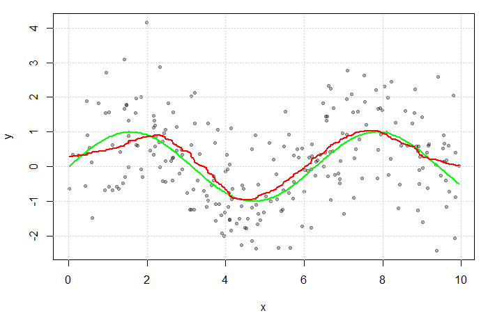
The red line is the result of estimating with a Gaussian kernel and arbitrarily selected bandwidth of  . The green line represents the true function
  .
.
 be a random variable with a continuous distribution function (CDF)
  and probability density function (PDF)
![\[f(x) = \frac{d}{dx} F(x)\]](https://statisticelle.com/wp-content/ql-cache/quicklatex.com-b7f63dc97bf17d7fd7215a8e571dc414_l3.png "Rendered by QuickLaTeX.com")
 . Estimation of
 ![\[ \hat{Pr}(C = c | X = x_0) = \frac{\hat{\pi}_c \hat{f}_{c}(x_0)}{\sum_{k=1}^{C} \hat{\pi}_{k} \hat{f}_{k}(x_0)} \]](https://statisticelle.com/wp-content/ql-cache/quicklatex.com-ec4bde07d3f9cbbb654aca700939e681_l3.png "Rendered by QuickLaTeX.com")