Statistics Archives • Page 2 of 3 • Statisticelle

U-, V-, and Dupree statistics

To start, I apologize for this blog’s title but I couldn’t resist referencing to the Owen Wilson classic You, Me, and Dupree – wow! The other gold-plated candidate was U-statistics and You. Please, please, hold your applause.

My previous blog post defined statistical functionals as any real-valued function of an unknown CDF, $T(F)$ , and explained how plug-in estimators could be constructed by substituting the empirical cumulative distribution function (ECDF) $\hat{F}_{n}$ for the unknown CDF $F$ . Plug-in estimators of the mean and variance were provided and used to demonstrate plug-in estimators’ potential to be biased.

$\hat{\mu} = \mathbb{E}_{\hat{F}_n}[X] = \sum_{i=1}^{n} X_i P(X = X_i) = \frac{1}{n} \sum_{i=1}^{n} X_i = \bar{X}_{n}$

$\hat{\sigma}^{2} = \mathbb{E}_{\hat{F}_{n}}[(X- \mathbb{E}_{\hat{F}_n}[X])^2] = \mathbb{E}_{\hat{F}_n}[(X - \bar{X}_{n})^2] = \frac{1}{n} \sum_{i=1}^{n} (X_i - \bar{X}_{n})^2.$

Statistical functionals that meet the following two criteria represent a special family of functionals known as expectation functionals:

1) $T(F)$ is the expectation of a function $g$ with respect to the distribution function $F$ ; and

$T(F) = \mathbb{E}_{F} ~g(X)$

2) the function $g(\cdot)$ takes the form of a symmetric kernel.

Expectation functionals encompass many common parameters and are well-behaved. Plug-in estimators of expectation functionals, named V-statistics after von Mises, can be obtained but may be biased. It is, however, always possible to construct an unbiased estimator of expectation functionals regardless of the underlying distribution function $F$ . These estimators are named U-statistics, with the “U” standing for unbiased.

This blog post provides 1) the definitions of symmetric kernels and expectation functionals; 2) an overview of plug-in estimators of expectation functionals or V-statistics; 3) an overview of unbiased estimators for expectation functionals or U-statistics.

Continue reading U-, V-, and Dupree statistics

Using a DAG to simulate data with the dagR library

Directed acyclic graphs (DAGs), and causal graphs in general, provide a framework for making assumptions explicit and identifying confounders or mediators of the relationship between the exposure of interest and outcome that need to be adjusted for in analysis. Recently, I ran into the need to generate data from a DAG for a paper I am writing with my peers Kevin McIntyre and Joshua Wiener. After a quick Google search, I was pleasantly surprised to see there were several options to do so. In particular, the dagR library provides “functions to draw, manipulate, [and] evaluate directed acyclic graphs and simulate corresponding data”.

Besides dagR‘s reference manual, a short letter published in Epidemiology, and a limited collection of examples, I couldn’t find too many resources regarding how to use the functionality provided by dagR. The goal of this blog post is to provide an expository example of how to create a DAG and generate data from it using the dagR library.

To simulate data from a DAG with dagR, we need to:

Create the DAG of interest using the dag.init function by specifying its nodes (exposure, outcome, and covariates) and their directed arcs (directed arrows to/from nodes).
Pass the DAG from (1) to the dag.sim function and specify the number of observations to be generated, arc coefficients, node types (binary or continuous), and parameters of the node distributions (Normal or Bernoulli).

For this tutorial, we are going to try to replicate the simple confounding/common cause DAG presented in Figure 1b as well as the more complex DAG in Figure 2a of Shier and Platt’s (2008) paper, Reducing bias through directed acyclic graphs.

library(dagR)
set.seed(12345)

Continue reading Using a DAG to simulate data with the dagR library

Parametric vs. Nonparametric Approach to Estimations

Parametric statistics assume that the unknown CDF $F$ belongs to a family of CDFs characterized by a parameter (vector) $\theta$ . As the form of $F$ is assumed, the target of estimation is its parameters $\theta$ . Thus, all uncertainty about $F$ is comprised of uncertainty about its parameters. Parameters are estimated by $\hat{\theta}$ , and estimates are be substituted into the assumed distribution to conduct inference for the quantities of interest. If the assumed distribution $F$ is incorrect, inference may also be inaccurate, or trends in the data may be missed.

To demonstrate the parametric approach, consider $n = 100$ independent and identically distributed random variables $X_1, …, X_n$ generated from an exponential distribution with rate $\lambda = 2$ . Investigators wish to estimate the 75 $^{th}$ percentile and erroneously assume that their data is normally distributed. Thus, $F$ is assumed to be the Normal CDF but $\mu$ and $\sigma^2$ are unknown. The parameters $\mu$ and $\sigma$ are estimated in their typical way by $\bar{x}$ and $\sigma^2$ , respectively. Since the normal distribution belongs to the location-scale family, an estimate of the $p^{th}$ percentile is provided by,

$x_p = \bar{x} + s\Phi^{-1}(p)$

where $\Phi^{-1}$ is the standard normal quantile function, also known as the probit.

set.seed(12345)
library(tidyverse, quietly = T)

# Generate data from Exp(2)
x <- rexp(n = 100, rate = 2)

# True value of 75th percentile with rate = 2
true <- qexp(p = 0.75, rate = 2) 
true

## [1] 0.6931472

# Estimate mu and sigma
xbar <- mean(x)
s    <- sd(x)

# Estimate 75th percentile assuming mu = xbar and sigma = s
param_est <- xbar + s * qnorm(p = 0.75)
param_est

## [1] 0.8792925

The true value of the 75 $^{th}$ percentile of $\text{Exp}(2)$ is 0.69 while the parametric estimate is 0.88.

Nonparametric statistics make fewer distributions about the unknown distribution $F$ , requiring only mild assumptions such as continuity or the existence of specific moments. Instead of estimating parameters of $F$ , $F$ itself is the target of estimation. $F$ is commonly estimated by the empirical cumulative distribution function (ECDF) $\hat{F}$ ,

$\hat{F}(x) = \frac{1}{n} \sum_{i=1}^{n} \mathbb{I}(X_i \leq x).$

Any statistic that can be expressed as a function of the CDF, known as a statistical functional and denoted $\theta = T(F)$ , can be estimated by substituting $\hat{F}$ for $F$ . That is, plug-in estimators can be obtained as $\hat{\theta} = T(\hat{F})$ .

Continue reading Parametric vs. Nonparametric Approach to Estimations

Kernel Regression

Motivation

For observed pairs $(x_i, y_i)$ , $i = 1, …, n$ , the relationship between $x$ and $y$ can be defined generally as

$y_i = m(x_i) + \varepsilon_i$

where $f(x_i) = E[y_i | x = x_i]$ and $\varepsilon_i \stackrel{iid}{\sim} (0, \sigma^2)$ . If we are unsure about the form of $m(\cdot)$ , our objective may be to estimate $m(\cdot)$ without making too many assumptions about its shape. In other words, we aim to “let the data speak for itself”.

Simulated scatterplot of $y = f(x) + \epsilon$ . Here, $x \sim Uniform(0, 10)$ and $\epsilon \sim N(0, 1)$ . The true function $f(x) = sin(x)$ is displayed in green.

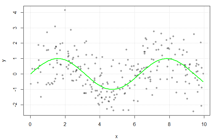
Non-parametric approaches require only that $m(\cdot)$ be smooth and continuous. These assumptions are far less restrictive than alternative parametric approaches, thereby increasing the number of potential fits and providing additional flexibility. This makes non-parametric models particularly appealing when prior knowledge about $m(\cdot)$ ‘s functional form is limited.

Estimating the Regression Function

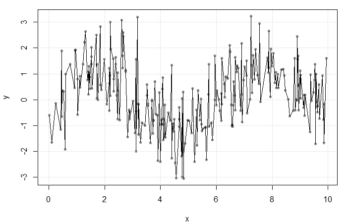
If multiple values of $y$ were observed at each $x$ , $f(x)$ could be estimated by averaging the value of the response at each $x$ . However, since $x$ is often continuous, it can take on a wide range of values making this quite rare. Instead, a neighbourhood of $x$ is considered.

Result of averaging $y_i$ at each $x_i$ . The fit is extremely rough due to gaps in $x$ and low $y$ frequency at each $x$ .

Define the neighbourhood around $x$ as $x \pm \lambda$ for some bandwidth $\lambda > 0$ . Then, a simple non-parametric estimate of $m(x)$ can be constructed as average of the $y_i$ ‘s corresponding to the $x_i$ within this neighbourhood. That is,

(1) $\begin{equation*} \hat{f}_{\lambda}(x) = \frac{\sum_{n} \mathbb{I}(|x - x_i| \leq \lambda)~ y_i}{\sum_{n} \mathbb{I}(|x - x_i| \leq \lambda)} = \frac{\sum_n K\left( \frac{x - x_i}{\lambda} \right) y_i}{\sum_n K\left( \frac{x - x_i}{\lambda} \right) } \end{equation*}$

where

$K(u) = \begin{cases} \frac{1}{2} & |u| \leq 1 \\ 0 & \text{o.w.} \end{cases}$

is the uniform kernel. This estimator, referred to as the Nadaraya-Watson estimator, can be generalized to any kernel function $K(u)$ (see my previous blog bost). It is, however, convention to use kernel functions of degree $\nu = 2$ (e.g. the Gaussian and Epanechnikov kernels).

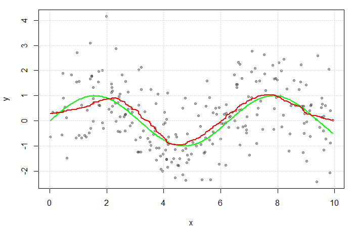
The red line is the result of estimating $f(x)$ with a Gaussian kernel and arbitrarily selected bandwidth of $\lambda = 1.25$ . The green line represents the true function $sin(x)$ .

Continue reading Kernel Regression